In this blog post, I will demonstrate how I applied a reconstruction convolutional autoencoder model to detect quality issues of sensor data. I also show that a small percentage of anomalous data points can result in a disproportionately large percentage of downstream calculations being inaccurate.
Introduction
Historically, the objective of detecting anomalies and identifying patterns of abnormal behavior in metering data was to quickly identify when production equipment is not functioning as intended. This can help the manufacturers to prevent downtime, reduce the time and cost of maintenance and repair, and minimize the impact on the production line, thus improving the overall quality of the final product and the overall equipment efficiency. However, the focus of this blog post is accurate measuring of energy use in production processes: sensors and meters are sources of the primary data on the energy consumption of production equipment; thus, if the production equipment is experiencing anomalies or the data collection infrastructure is not functioning correctly, the data collected will not accurately reflect actual energy consumption. This can result in inaccurate calculations of energy use and can affect the accuracy of any calculations based on this data, such as organizational carbon footprint and product carbon footprint. By detecting and flagging anomalous data points, it is possible to adjust the calculations for the corresponding time window, resulting in a more precise measurement of energy use.
Setup
In what follows, I will use synthesised data of electric current for an engine working in a batch process manufacturing line. See one of the previous blog posts, Applying OPP Principles to Manufacturing Analytics Testing Data Generation, for more details. The dataset includes minutely data for the period August 06 to September 07, 2022:
I use the part of the data before the CUT_POINT for training and the rest of the data for testing to see if the sudden jump ups in the data is detected as an anomaly:
CUT_POINT = '2022-08-09 18:00:00'
training_df = generated_time_series.loc[:CUT_POINT].copy()
testing_df = generated_time_series.loc[CUT_POINT:].copy()
Note: as I want the missing data points be also detected as anomalous, I will fill them in with the maximum of observed electric current values before feeding them into the autoencoder.
Let’s import the required libraries:
import numpy as np
import pandas as pd
import plotly.graph_objs as go
from matplotlib import pyplot as plt
from tensorflow.keras.models import Sequential
from tensorflow.keras.layers import Input, Conv1D, Dropout, Conv1DTranspose
from tensorflow.keras.optimizers import Adam
Anomaly Detector
To implement the task, I introduced a custom class called AnomalyDetector, which includes methods for sequence generation1, model building, training, and others. The __init__ method of the class takes the training and the testing datasets and the number of data points for generating sequences as parameters. Note: the data has its inner structure and periodicity of approximately 150 timestamps (the nominal batch duration plus the time window between batches according to our hypothetical production process specification), thus, to create sequences, I chose to combine TIME_STEPS=150 contiguous data values.
TIME_STEPS = 150

class AnomalyDetector:

    def __init__(
        self,
        training_data: pd.DataFrame,
        testing_data: pd.DataFrame,
        time_steps_number: int
    ):
        """
        :param training_df: a pandas minutely time series dataframe with 'time' as index
        and 'current' as sensor values, used for training
        :param testing_df: a pandas minutely time series dataframe with 'time' as index
        and 'current' as sensor values, used for testing
        :param time_steps_number: sequences length
        """
        self.training_df = training_data
        self.testing_df = testing_data
        self.time_steps_number = time_steps_number
Data preparation
To prepare the data for sequence generation, I first extract the data values from the time series and then normalize them. We use the training mean and standard deviation to normalize the validation and test timeseries. Then I construct training and testing sequences.
    def normalize_data(self):
        self.training_mean = self.training_df.mean()
        self.training_std = self.training_df.std()
        self.normalized_training_df = (
            self.training_df - self.training_mean
        ) / self.training_std
        self.normalized_testing_df = (
            self.testing_df - self.training_mean
        ) / self.training_std
        print(f"Number of training samples: {len(self.normalized_training_df)}")
        print(f"Number of testing samples: {len(self.normalized_testing_df)}")

    def __generate_sequences(self, values: np.array):
        # Generated training sequences for use in the model.
        output = []
        for i in range(len(values) - self.time_steps_number + 1):
            output.append(values[i : (i + self.time_steps_number)])
        return np.stack(output)

    def generate_training_sequences(self):
        self.training_sequences = self.__generate_sequences(
            self.normalized_training_df.values
        )
        print(f"Training input shape: {self.training_sequences.shape}")

    def generate_testing_sequences(self):
        self.testing_sequences = self.__generate_sequences(
            self.normalized_testing_df.values
        )
        print(f"Testing input shape: {self.testing_sequences.shape}")
Building the model
Convolutional reconstruction autoencoder
To detect anomalies in batch process manufacturing data, I employed a convolutional reconstruction autoencoder model for sequenced data. It is a type of neural network that analyzes the sequential structure of the input data and learns to encode and decode sequential data by extracting and reconstructing relevant features from the input sequence. During training, the model minimizes the difference between the input and output sequences, and the resulting reconstructed sequences for the testing data can be compared to the original ones to detect anomalies. There have been several studies and publications that have demonstrated the effectiveness of using autoencoders for anomaly detection in various process manufacturing related domains2.
Architecture
The convolutional architecture is thought to be particularly suited to data, where local features and relationships between adjacent data points are important. The classical architecture of a convolutional reconstruction autoencoder model consists of an encoder and a decoder, where the encoder includes of one or more convolutional layers followed by one or more pooling layers, which reduce the spatial dimensions of the input, and the decoder includes of one or more transposed convolutional layers followed by one or more upsampling layers, which reconstruct the original input from the low-dimensional representation created by the encoder. The “bottleneck” layer is typically a fully connected or dense layer that connects the encoder and decoder. The goal is to learn a compressed representation of the input data in the bottleneck layer, which can be used for anomaly detection or other downstream tasks. I’ve ended up experimenting with removing the central layer of the classical CNN model and found that the model still performed well without it3, so I implemented the following basic architecture (see the create_model method below):
- After the
Inputlayer, the model includes two 1D convolutional layers and twoConv1DTransposelayers, with one Droput layer between them; - The use of Dropout layers helps to prevent overfitting of the model to the training data;
- Finally, the output layer is a
Conv1DTransposelayer with the filter parameter value of one to produce final one-dimensionsl output.
The model takes two parameters, sequence_length and num_features. In our case, sequence_length equals TIME_STEPS and num_features takes the value of one (the electric current values); both parameters are stored in the shape instance of the sequence tensor.
    def create_model(self):
        # define the model
        model = Sequential()
        # add layers to model
        model.add(Input(shape=(
            self.training_sequences.shape[1], self.training_sequences.shape[2]
        )))
        model.add(Conv1D(filters=30, kernel_size=7, padding="same", activation="relu"))
        model.add(Dropout(rate=0.2))
        model.add(Conv1D(filters=15, kernel_size=7, padding="same", activation="relu"))
        model.add(Conv1DTranspose(
            filters=15, kernel_size=7, padding="same", activation="relu"
        ))
        model.add(Dropout(rate=0.2))
        model.add(Conv1DTranspose(
            filters=30, kernel_size=7, padding="same", activation="relu"
        ))
        model.add(Conv1DTranspose(filters=1, kernel_size=7, padding="same"))
        # add compiler
        optimizer = Adam(learning_rate=0.001)
        model.compile(optimizer=optimizer, loss='mse')
        self.model = model
        print(self.model.summary())
Using padding="same" parameter in the convolutional layers ensures that the output feature maps have the same length as the input time series by padding zeros to the edges of the input sequence if necessary. This is important for preserving the temporal structure of the data and allowing the model to learn meaningful patterns across the entire sequence. Without padding, the convolutional layers would reduce the length of the sequence, which could result in loss of information and reduced model performance.
Using the rectified linear unit (ReLU) activation function, which besides preventing the vanishing gradient problem during training, helps to ensure that output values are always non-negative (since we are working with non-negative values).
30 filters with a width of 7 time steps (minutes) are applied to the input sequences. This configuration can be, of course, modified, e.g., with the help of automated hyper-parameter tuning, which I leave beyond the scope of this blog post.4
I wanted to leverage the MSE loss function for our time series autoencoder as a straightforward choice: as a more computationally efficient one for gradient-based optimization methods like Adam, and for putting a higher weight on larger errors.
Training the model
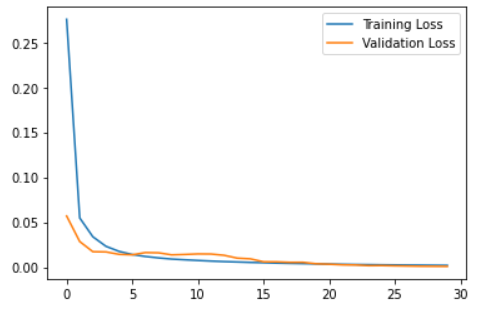
When training the model, I used batches of 128 samples in 30 epochs and set aside 10% of the data for validation. Then I plot the resulting training and validation loss to see how the training went.
    def train_model(self, epochs=30, batch_size=128, validation_split=0.1):
        # fit model
        history = self.model.fit(
            self.training_sequences,
            self.training_sequences,
            epochs=epochs,
            batch_size=batch_size,
            validation_split=validation_split,
        )
        self.history = history
        # plot losses
        plt.plot(self.history.history["loss"], label="Training Loss")
        plt.plot(self.history.history["val_loss"], label="Validation Loss")
        plt.legend()
        plt.show()
Anomaly detection
The anomalies are detected by determining how well our model can reconstruct the input data. To this end I:
- Get reconstruction error threshold;
- Compare recontruction;
- Run the model on the testing data;
- Label anomalies;
- Find anomalous data points in the original testing data.
Get reconstruction error threshold
- Find
MAEloss on training samples (at this step, we want to treat all errors equally). - Find max
MAEloss value. This is the worst our model has performed trying to reconstruct a sample. We will make this value the threshold for anomaly detection. - If the reconstruction loss for a sample is greater than the stated value then we can infer that the model is seeing a pattern that is not familiar to it. We will label this sample as an anomaly.
    def get_reconstruction_error_threshold(self):
        # calculate predictions
        self.train_predictions = self.model.predict(self.training_sequences)
        # calculte MAE loss
        self.train_mae_loss = np.mean(
            np.abs(self.train_predictions - self.training_sequences), axis=1
        )
        # get reconstruction loss threshold
        self.threshold = np.max(self.train_mae_loss)
        # plot the distribution of the train MAE losses
        plt.hist(self.train_mae_loss, bins=50)
        plt.xlabel("Train MAE loss")
        plt.ylabel("No of samples")
        plt.show()
        # print out the threshold
        print(f"Reconstruction error threshold: {self.threshold}")
Compare recontruction
To grasp a visual impression of how the things worked out, I added a method to plot one of the sequences of our training dataset and the reconstructed sequence.
    def plot_one_reconstructed_training_sequence(self, sequence_num: int):
        """Checks out visualy how reconstruction worked"""
        plt.plot(self.training_sequences[sequence_num], label="Training sample")
        plt.plot(self.train_predictions[sequence_num], label="Predicted sample")
        plt.legend()
        plt.show()
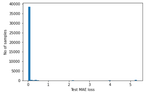
Run the model on the testing data
Then I added a method for reconstructing the testing sequences.
    def get_reconstructed_testing_sequences(self):
        # calculate predictions
        self.testing_predictions = self.model.predict(self.testing_sequences)
        # calculate MAE loss
        self.test_mae_loss = np.mean(
            np.abs(self.testing_predictions - self.testing_sequences), axis=1
        )
        # plot the distribution of the test MAE losses
        plt.hist(self.test_mae_loss, bins=50)
        plt.xlabel("Test MAE loss")
        plt.ylabel("No of samples")
        plt.show()
Label anomalies
Anomalies are defined as testing samples with testing MAE loss above the reconstruction error threshold.
    def mark_anomalous_samples(self):
        # Detect all the samples which are anomalies.
        self.anomalies = self.test_mae_loss > self.threshold
        print(f"Number of anomaly samples: {np.sum(self.anomalies)}")
        print(f"Indices of anomaly samples: {np.where(self.anomalies)[0]}")
Find anomalous data points in the original testing data
To determine the anomalous data points, I check each data point on being presented in anomalous sequences: data point i is an anomaly if samples [(i - timesteps + 1) to (i)] are anomalies.
    def mark_anomalous_data_points(self):
        anomalous_data_indices = []
        for data_idx in range(
          self.time_steps_number - 1,
          len(self.normalized_testing_df) - self.time_steps_number + 1
        ):
            if np.all(self.anomalies[data_idx - 149 : data_idx]):
                anomalous_data_indices.append(data_idx)
        self.anomalous_data_indices = anomalous_data_indices
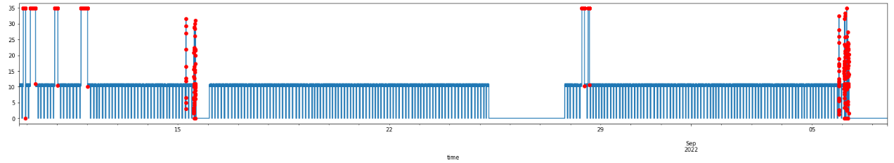
Plot anomalies
I introduce two methods, to plot one of the testing reconstructed sequences and to overlay the anomalies on the original test data plot.
    def plot_one_reconstructed_testing_sequence(self, sequence_num: int):
        """Checks out visualy how reconstruction worked"""
        plt.plot(self.testing_sequences[sequence_num], label="Testing sample")
        plt.plot(self.testing_predictions[sequence_num], label="Predicted sample")
        plt.legend()
        plt.show()

    def visualize_anomalies(self, start_index: int, end_index: int):
        df_subset = self.testing_df.iloc[self.anomalous_data_indices]
        fig, ax = plt.subplots(figsize=(28,4))
        self.testing_df[start_index:end_index].plot(legend=False, ax=ax)
        start_ts = self.testing_df.iloc[start_index].name
        end_ts = self.testing_df.iloc[end_index].name
        df_subset[start_ts:end_ts].plot(
            legend=False, ax=ax, color="r", marker='o', linestyle='None'
        )
        plt.show()
Construct labeled testing dataset
Finally, after fetching the anamalous data point indices, I add labels to the testing dataset.
    def construct_labeled_testing_time_series(self):
        df = self.testing_df.copy()
        df.reset_index(inplace=True)
        df['anomaly'] = False
        df.loc[self.anomalous_data_indices, 'anomaly'] = True
        self.testing_df_labeled = df.set_index('time')
        self.time_series_dqr = (
            1 - self.testing_df_labeled.anomaly.sum()/len(self.testing_df_labeled)
        )*100
Running the model
To demonstrate how the anomaly detector works, I explicitly run each method of the class. As previously mentioned, I want to detect missing data points as anomalous as well, so I fill them in with the maximum value of the current data.
ad = AnomalyDetector(
    training_df,
    testing_df.fillna(testing_df['current'].apply('max')),
    TIME_STEPS
)
ad.normalize_data()
ad.generate_training_sequences()
ad.generate_testing_sequences()
ad.create_model()
ad.train_model()
ad.get_reconstruction_error_threshold()
ad.get_reconstructed_testing_sequences()
ad.mark_anomalous_samples()
ad.mark_anomalous_data_points()
ad.construct_labeled_testing_time_series()

Number of training samples: 5311
Number of testing samples: 41409
Training input shape: (5162, 150, 1)
Testing input shape: (41260, 150, 1)
Model: "sequential_1"
_________________________________________________________________
 Layer (type)                Output Shape              Param #
=================================================================
 conv1d_44 (Conv1D)          (None, 150, 30)           240

 dropout_43 (Dropout)        (None, 150, 30)           0

 conv1d_45 (Conv1D)          (None, 150, 15)           3165

 conv1d_transpose_64 (Conv1D  (None, 150, 15)          1590
 Transpose)

 dropout_44 (Dropout)        (None, 150, 15)           0

 conv1d_transpose_65 (Conv1D  (None, 150, 30)          3180
 Transpose)

 conv1d_transpose_66 (Conv1D  (None, 150, 1)           211
 Transpose)

=================================================================
Total params: 8,386
Trainable params: 8,386
Non-trainable params: 0
_________________________________________________________________
None
Epoch 1/30
37/37 [==============================] - 3s 59ms/step
- loss: 0.2756 - val_loss: 0.0570
Epoch 2/30
37/37 [==============================] - 2s 49ms/step
- loss: 0.0548 - val_loss: 0.0286
Epoch 3/30
37/37 [==============================] - 2s 48ms/step
- loss: 0.0339 - val_loss: 0.0173
Epoch 4/30
37/37 [==============================] - 2s 48ms/step
- loss: 0.0233 - val_loss: 0.0171
Epoch 5/30
37/37 [==============================] - 2s 48ms/step
- loss: 0.0176 - val_loss: 0.0144
Epoch 6/30
37/37 [==============================] - 2s 48ms/step
- loss: 0.0142 - val_loss: 0.0139
Epoch 7/30
37/37 [==============================] - 2s 48ms/step
- loss: 0.0120 - val_loss: 0.0163
Epoch 8/30
37/37 [==============================] - 2s 49ms/step
- loss: 0.0104 - val_loss: 0.0161
Epoch 9/30
37/37 [==============================] - 2s 49ms/step
- loss: 0.0091 - val_loss: 0.0138
Epoch 10/30
37/37 [==============================] - 2s 52ms/step
- loss: 0.0083 - val_loss: 0.0142
Epoch 11/30
37/37 [==============================] - 2s 51ms/step
- loss: 0.0076 - val_loss: 0.0148
Epoch 12/30
37/37 [==============================] - 2s 49ms/step
- loss: 0.0069 - val_loss: 0.0147
Epoch 13/30
37/37 [==============================] - 2s 48ms/step
- loss: 0.0063 - val_loss: 0.0133
Epoch 14/30
37/37 [==============================] - 2s 50ms/step
- loss: 0.0059 - val_loss: 0.0102
Epoch 15/30
37/37 [==============================] - 2s 48ms/step
- loss: 0.0054 - val_loss: 0.0093
Epoch 16/30
37/37 [==============================] - 2s 48ms/step
- loss: 0.0050 - val_loss: 0.0061
Epoch 17/30
37/37 [==============================] - 2s 48ms/step
- loss: 0.0046 - val_loss: 0.0060
Epoch 18/30
37/37 [==============================] - 2s 53ms/step
- loss: 0.0043 - val_loss: 0.0055
Epoch 19/30
37/37 [==============================] - 2s 53ms/step
- loss: 0.0041 - val_loss: 0.0055
Epoch 20/30
37/37 [==============================] - 2s 49ms/step
- loss: 0.0038 - val_loss: 0.0039
Epoch 21/30
37/37 [==============================] - 2s 52ms/step
- loss: 0.0035 - val_loss: 0.0034
Epoch 22/30
37/37 [==============================] - 2s 52ms/step
- loss: 0.0033 - val_loss: 0.0027
Epoch 23/30
37/37 [==============================] - 2s 46ms/step
- loss: 0.0031 - val_loss: 0.0025
Epoch 24/30
37/37 [==============================] - 2s 47ms/step
- loss: 0.0029 - val_loss: 0.0018
Epoch 25/30
37/37 [==============================] - 2s 47ms/step
- loss: 0.0027 - val_loss: 0.0019
Epoch 26/30
37/37 [==============================] - 2s 46ms/step
- loss: 0.0026 - val_loss: 0.0016
Epoch 27/30
37/37 [==============================] - 2s 50ms/step
- loss: 0.0025 - val_loss: 0.0014
Epoch 28/30
37/37 [==============================] - 2s 52ms/step
- loss: 0.0024 - val_loss: 0.0012
Epoch 29/30
37/37 [==============================] - 2s 48ms/step
- loss: 0.0022 - val_loss: 0.0011
Epoch 30/30
37/37 [==============================] - 2s 49ms/step
- loss: 0.0021 - val_loss: 9.7198e-04
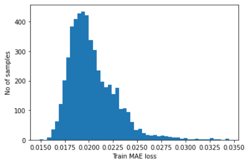
Reconstruction error threshold: 0.03448834298971466
Number of anomaly samples: 2853
Indices of anomaly samples: [   44    45    46 ... 39556 39557 39558]
Reviewing the results
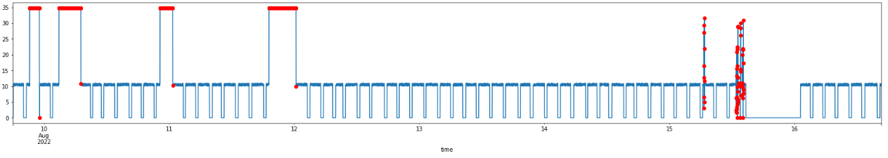
Now, I can visualize the detected anomalous data points!
ad_filled.visualize_anomalies(0,-1)
And in more details:
ad_filled.visualize_anomalies(0,10000)
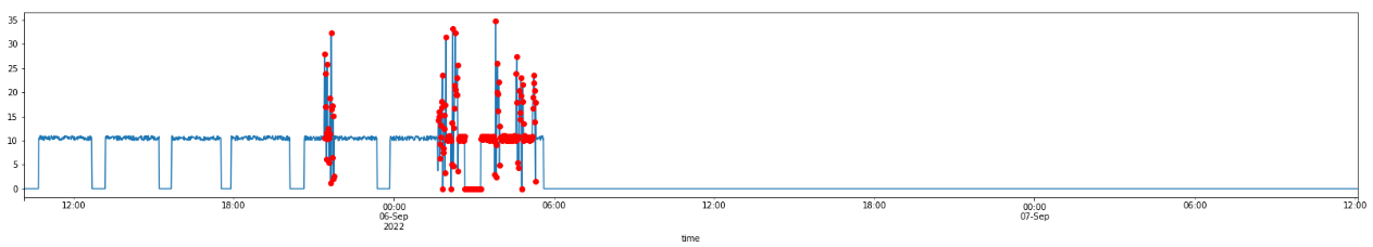
ad_filled.visualize_anomalies(-3000,-1)
Finally, let’s print out an example of the labeled timeseries and see the estimated time series data quality for the testing subset:
ad.testing_df_labeled[190:195]

                        current	        anomaly
time
2022-08-09 21:10:00	10.730894	False
2022-08-09 21:11:00	10.897367	False
2022-08-09 21:12:00	10.083670	False
2022-08-09 21:13:00	34.825259	True
2022-08-09 21:14:00	34.825259	True

print(f"{ad.time_series_dqr = :.1f}%")
ad.time_series_dqr = 96.7%
Thus, I have successfully detected all the anomalies in the data, both the malfunctioning equipment and what seems to be issues within the data collection infrastructure. An interesting observation is that, when considering each data point of the timeseries on its own, less than 4% of the dataset can be considered as failed. In the last section, to demonstrate how the detected anomalies actually impact the quality of the batch data, I implemented a simple batch data analyzer.
Batch Analyzer
I introduced another class, called BatchAnalyzer, which includes methods for generating raw data on batches and for extracting timings, like batch duration and time window duration between batches, and a method to calculate the resulting batch data quality rating5. In addition to the labeled timeseries, it takes two parameters: nominal expected batch duration (in minutes) and the number of batches produced within the given period, as documented in the ERP system.
class BatchAnalyzer:

    def __init__(
        self,
        input_df: pd.DataFrame,
        batch_spec_duration: int,
        batch_number_in_erp: int
    ):
        """
        :param input_df: a pandas minutely time series dataframe with 'time'
        as index and 'current' and 'anomaly' columns.
        """
        self.input_df = input_df.copy()
        self.batch_spec_duration = batch_spec_duration
        self.batch_number_in_erp = batch_number_in_erp

    def __check_input_df(self):
        column_names = self.input_df.columns.to_list() == ['current', 'anomaly']
        time_index = self.input_df.index.name == 'time'
        if column_names and time_index:
            return True

    def generate_raw_batch_data(self):
        df = self.input_df.copy()
        if self.__check_input_df():
            # Add a column indicating if the current is non-zero
            df['current_on'] = df['current'].apply(lambda x: False if x == 0 else True)
            # Add a column indicating if the current is zero
            df['current_off'] = df['current'].apply(lambda x: True if x == 0 else False)
            # Add a column indicating if the current state changed from the previous row
            df['state_changed'] = df['current_on'].ne(df['current_on'].shift())
            df['state_changed_to_on'] = np.where(
                df['current']* df['state_changed'],
                True,
                False
            )
            # Add a column indicating the batch number
            df['batch_number'] = df['state_changed_to_on'].cumsum()

            self.raw_batch_data = df
        else:
            print(f"Unacceptable dataframe, proper dataframe has `time` index, \
            and `current` and `anomaly` columns.")

    def extract_raw_batch_timings(self):
        df = self.raw_batch_data.copy().reset_index()
        # create a dataframe with batch numbers, their start time and end time
        batch_df = pd.pivot_table(
            df, values = ['time', 'anomaly'],
            columns = 'current_on',
            index = 'batch_number',
            aggfunc = {'time': ['min', 'max'], 'anomaly': ['max']}
        )
        batch_df.columns = [
            'window_anomaly',
            'batch_anomaly',
            'window_end_time',
            'batch_end_time',
            'window_start_time',
            'batch_start_time'
        ]
        batch_df = batch_df[[
            'batch_start_time',
            'batch_end_time',
            'window_start_time',
            'window_end_time',
            'batch_anomaly',
            'window_anomaly'
        ]]
        batch_df['batch_duration'] = (
            batch_df.batch_end_time - batch_df.batch_start_time
        ).astype('timedelta64[m]')
        batch_df['window_duration'] = (
            batch_df.window_end_time - batch_df.window_start_time
        ).astype('timedelta64[m]')

        self.raw_batch_timing_data = batch_df

    def calculate_batch_data_quality_rating(self):
        self.batch_dqr = (self.raw_batch_timing_data.query(
            'batch_duration > @self.batch_spec_duration*.75 \
            & batch_duration < @self.batch_spec_duration*1.25'
        ).batch_duration.sum()/self.batch_number_in_erp/self.batch_spec_duration)*100
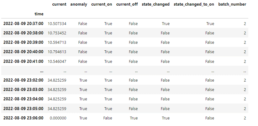
The raw_batch_data dataframe includes the initial labeled timeseries with additional columns indicating the current status changes and attributed batch numbers, e.g.:
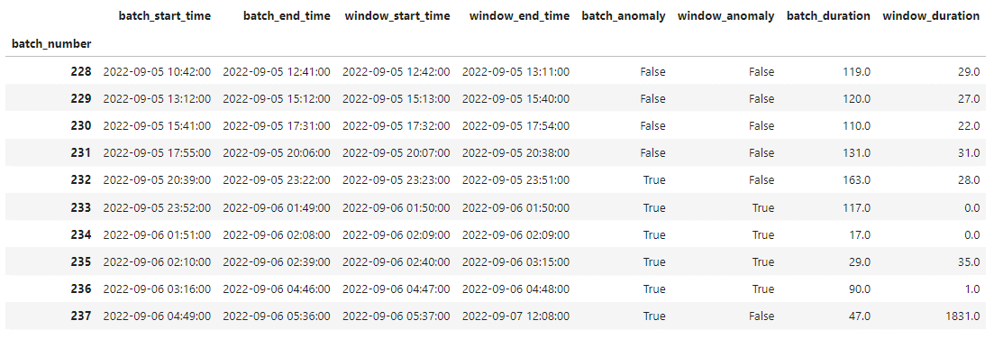
The raw_batch_timing_data dataframe is a pivot table presenting batch_start_time, batch_end_time, window_start_time, window_end_time, batch_anomaly, window_anomaly, batch_duration, and window_duration values for each extracted batch, e.g.:
I used the following script to run the batch analyzer:
ERP_BATCH_NUM = 241
BATCH_SPEC_DURATION = 120  # BATCH_SPEC_DURATION = TIME_STEPS - WINDOW_SPEC_DURATION

bc = BatchAnalyzer(ad_filled.testing_df_labeled, BATCH_SPEC_DURATION, ERP_BATCH_NUM)
bc.generate_raw_batch_data()
bc.extract_raw_batch_timings()
bc.calculate_batch_data_quality_rating()
Let’s check the resulting batch data quality rating:
print(f"{bc.batch_dqr = :.1f}%")
bc.batch_dqr = 90.0%
It turns out that less than 4% of anomalous data points can result in 10% of batches being with inaccurately detected.
Conclusions
In this blog post, I demonstrated a successful implementation of a sequence-based convolutional autoencoder for detecting anomalies in timeseries data, specifically focusing on identifying production equipment malfunctions and data collection issues. Even with a simple model, I achievde accurate enough anomaly detection. I also showed how the detected anomalies in the raw timeseries can be used in labeling the batch data and how they impact the overall quality rating of the batch data. Our work highlights the potential of using advanced machine learning techniques to enhance the primary data fed into downstream calculations, such as product carbon footprint.
1 In what follows, I apply a sequence-based model. It learns to encode and decode sequential data by extracting and reconstructing relevant features from the input sequences, which are constructed from a given timeseries. The sequence generation is performed using a sliding window approach. The initial timeseries is divided into overlapping windows of a specified length, and each window is treated as a sequence of data points. The length of the window, defined by the TIME_STEPS parameter, determines the length of the sequence (150 data points in our case), and the amount of overlap between adjacent windows can also be specified (we use one data point). By sliding the window along the time axis of the data, multiple sequences are generated from a single time series. These sequences are then fed into the convolutional reconstruction autoencoder model for training and the following for anomaly detection.
2 See, for example: Autoencoders for Anomaly Detection in an Industrial Multivariate Time Series Dataset. Tziolas et al. Eng. Proc. 2022, 18(1), 23; Anomaly Detection in Univariate Time-Series: a Surbey on the State-of-the-Art. Braei and Wagner. 2020; A Deep Neural Network for Unsupervised Anomaly Detection and Diagnosis in Multivariate Time Series Data. Zhang et al. 2018.
NOTE: In this case study, the signal has constant statistical properties, such as a constant mean and variance over time, and the underlying process generating the signal is stable, i.e., it can be considered a stationary time series, in which case a reconstruction convolutional autoencoder may be well-suited for modeling the signal and detecting anomalies or predicting future values. However, if the signal has time-varying statistical properties, such as cyclical or seasonal variations, trend changes, and other time-dependent effects, or the underlying production process generating the signal is changing, then it cannot be considered a stationary time series and other time series models, either statistical (such as statistical process control or wavelet analysis) or ML/AI (such as SVM or LSTM), may be applied to capture the complexity of the signal.
3 Removing the bottleneck layer is considered to be useful for some applications where the goal is not to reduce the dimensionality of the input data, but rather to reconstruct the original input with minimal distortion (see the link for deeper discussion of the needs and possible implementations).
4 The optimal number of filters and their width depends on various factors, such as the complexity of the input data, the desired level of abstraction, the available computational resources, and the specific task the model is being trained for. In general, one can start with a smaller number of filters and narrower filter widths and gradually increase their size and number based on the model’s performance and the complexity of the problem. In our case, the choice of filter size and the number of filters is based on my prior knowledge of the problem. In practice, hyperparameter tuning is an important step to determine the optimal configuration for a given problem.
5 Only for demonstrational purposes, we calculate the batch quality rating as the proportion of batches which length was within +-25% of the spec duration.
Copyright © 2022 Zheniya Mogilevski